Leveraging on transfer learning for image classification using Keras
Supercharge your image classification tasks by integrating large pre-trained deep learning models with very little effort.
Subscribe to our awesome Newsletter.

The task of image classification has persisted from the beginning of computer vision. There have been multiple breakthroughs over the years. Before the onset of Deep Learning, computer vision was heavily dependent on hardcoded mathematical formulas that worked on very specific use cases. With the advances in neural networks, convolutional neural networks (CNN) have become very efficient at image classification. Datasets like the Imagenet helped a lot in aiding the CNN learn features faster.
Transfer learning is a method to use models with pre-trained weights on large datasets like Imagenet. This is a very efficient method to do image classification because, we can use transfer learning to create a model that suits our use case. One important task that an image classification model needs to be good at is - they should classify images belonging to the same class and also differentiate between images that are different. Here we can leverage on the pre-trained model’s weights. These models have thousands of classes and can differentiate very well among all classes.
Depending on our dataset, we can use multiple methods in transfer learning. If our dataset is small and similar to the original dataset, we could use the pre-trained convnets as a fixed feature extractor. In this method, we remove the last fully connected layers. A fixed length vector is computed for every image and then a linear classifier is trained for the new dataset. Another method is to actually fine-tune the convnet by retraining the weights by continuing the back-propagation. In this tutorial, we will see the first method of removing the last layer and attaching our own classifier.
Let us consider a case where we have a dataset of flowers that we would like to classify as their respective types. You can download the dataset from here (This can be done programmatically as well). This dataset has 5 classes of flowers - Daisy, Dandelions, Sunflowers, Roses and Tulips. First and foremost we need convert the data into a format that is needed by the Keras function.
Preparing the data Our dataset has the images in their respective class folders. We need to split them into train, test and validation datasets.
| |
First, we get the class names from the flowers classes in the directory. Then we proceed to rename all the files with their class name appended with respective indices. Then we append them to the file_paths list along with the labels of each image.
Now, we need to split our dataset into train, test and validation. In each of the aforementioned folders, they need to have all the classes as folders. Then we proceed to copy the data from /flowers_photos folder into /data/train, /data/test and /data/validation.
| |
For the model to train, we have to one-hot encode the data. To achieve this, we use the LabelBinarizer from sklearn. After this, Stratified Shuffle Split from sklearn library to shuffle our data so that all similar data is not clustered together. Then we use the shutil inbuilt library to copy the files into respective folders. After this, the labels for train, test and validation are saved as a pickle for using them during training.
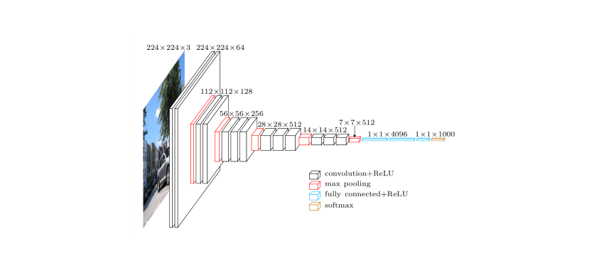
Training the model Now, we have to train the model with our dataset. First, from keras we import the pre-trained model of VGG16 with weights trained on imagenet. While loading, we include the argument include_top = False this will remove the 3 top fully connected layers. Be sure to update Keras to 2.0. Since the data set is small, we have to augment the images. Augmentation means that we have to apply different types of transformation. We are scaling the data between 1 to 255, with a image rotation range of 40 degrees along with a few other transformations.
| |
Keras has all this inbuilt so, we don’t need to worry about doing it manually using tools like opencv or scikit-image. ImageDataGenerator() has other arguments as well, you can use them if you need further augmentations. Then we proceed to create a generator with a resized image of 150 X 150 and saving the features as numpy arrays.
Before proceeding to train the model, we need to one hot encode the labels for the model to process. One hot encoding is a process to transform categorical features into a format that is more suitable for classification and regression problems. In this process we initialize an array with the shape (length of labels, number of classes). For the class that the label corresponds to labelled 1 and the remaining are 0.
| |
Adding our classification layers is very straightforward. We just stack them like a normal keras model. Then in the model.fit() method we provide the bottleneck features of both training and validation. Now that we have 5 classes, we will add our last layer as a classification layer.
| |
After this, the trained model weights are saved to disk for further usage. Here you can make the predictions as required. You could also continue to finetune the convnet to increase the accuracy of your predictions.
| |
Here is how we fared on training the model after 5 epochs. It can definitely do better. Let us know in the comment section if you have better ideas to improve the model.
If the dataset is larger and similar to the original dataset, you can train the last convolutional block as well. This will help in updating the weights of the network in accordance to the use case at hand. But a word of caution, make sure that the learning rate is very low to ensure that the learned weights of the network don’t undergo drastic changes. Also the optimizer for the network should preferably be Stochastic Gradient Descent (sgd) with a very low learning rate. Other optimization methods are not used because they would cause aggressive weight changes.
There are a lot of exciting use cases for using transfer learning. It can reduce your effort considerably while building a classification model, also you could integrate other mechanisms to perform more complex tasks like object detection.
So, that’s it from our side on transfer learning, now it’s upto you guys to try it and tell us how it goes!
